OPTIMIZING TRANSFORMER MODELS FOR PROFITABLE AND SLIPPAGE-RESISTANT HIGH-FREQUENCY TRADING
In algorithmic trading, achieving high predictive accuracy is crucial for staying ahead in volatile markets. This blog delves into the effectiveness of Transformer-based deep learning models for financial time series forecasting, showcasing their ability to identify intricate market trends. By utilizing multi-head attention mechanisms, normalization techniques, and advanced hyperparameter tuning, these models significantly improve prediction accuracy.
A comprehensive 180-day backtesting analysis evaluates profitability, risk management, and the impact of slippage, demonstrating a strong profit factor of 1.85. The results highlight the advantages of high-frequency trading strategies and the necessity of execution optimizations to minimize slippage and drawdowns. This study underscores the importance of adaptive trade execution strategies in maintaining long-term profitability in dynamic financial environments.
INTRODUCTION
In recent years, algorithmic trading has gained significant traction in financial markets, leveraging advanced machine learning techniques to enhance decision-making and execution efficiency. Among various deep learning models, Transformer-based architectures have demonstrated superior performance in capturing sequential dependencies within financial time series data. These models, originally designed for natural language processing (Vaswani et al., 2017), have been successfully adapted for time series forecasting, particularly in high-frequency trading and options market analysis.
Previous studies have explored the application of recurrent neural networks (RNNs) and long short-term memory (LSTM) networks for financial predictions (Fischer & Krauss, 2018). However, their limitations in handling long-range dependencies and computational inefficiencies have led to the adoption of Transformer-based models, which utilize self-attention mechanisms for better contextual learning (Zerveas et al., 2021). Moreover, hyperparameter optimization techniques have been introduced to fine-tune deep learning models, improving their adaptability and accuracy in real-time trading scenarios (Bergstra & Bengio, 2012).
Despite advancements, key challenges persist in the practical implementation of these models, including slippage impact, high drawdowns, and execution inefficiencies. This study aims to address these issues by optimizing a Transformer-based prediction model for options trading, with a focus on minimizing risk and maximizing profitability. The primary research question is: How can Transformer-based deep learning models be optimized to enhance profitability while mitigating slippage and drawdown risks in high-frequency options trading?
The hypothesis of this study posits that a well-optimized Transformer model, incorporating automated hyperparameter tuning and risk management techniques, can significantly improve trading performance by reducing execution inefficiencies and enhancing predictive accuracy.
The objective of this article is to present a comprehensive analysis of the proposed trading strategy, including model architecture, training methodology, backtesting results, and risk assessment. By integrating state-of-the-art deep learning approaches with robust trade execution strategies, this study aims to contribute to the ongoing advancements in algorithmic trading and financial forecasting.
PROJECT OVERVIEW
Technical Overview
Model Architecture – Transformer-Based Prediction
We leverage a Transformer-based deep learning model, which is highly effective in capturing sequential
dependencies within financial time series data. Our model is built with:
- Multi-Head Attention Layers – Allows the model to focus on different time frames.
- Layer Normalization & Batch Normalization – Improves training stability.
- L2 Regularization & Dropout – Reduces overfitting and enhances model generalization.
- Fully Connected Layers – Predicts the next price movements across four key values (open, high, low, close).
Hyperparameter Optimization & Training
Rather than manually selecting hyperparameters, we automate this process through optimization tools. This
technique fine-tunes:
- The number of attention heads and key dimensions – Optimizes pattern recognition.
- Activation functions and dropout rates – Improves overall performance.
- Optimizer settings – Fine-tunes learning rate, momentum, and gradient clipping for stability.
To avoid excessive training time and computational inefficiency, we implement early
stopping,
which prevents overfitting by halting training when performance plateaus.
We have created nearly 1000 models, leveraging auto-optimization methods to identify the
best-performing architecture. This iterative approach has allowed us to refine and continuously improve
our
model for optimal performance in options analysis.
TEST RESULTS
The objective of this backtesting analysis is to evaluate the profitability of the options buying strategy while minimizing drawdowns, ensuring an optimal balance between risk and reward.
Key findings from the backtest include a detailed analysis of each failure encountered during testing, with strategic adjustments implemented to enhance performance and minimize weaknesses.
The backtesting was performed for **180 days** (2024-06-03 09:15:00+00 to 2025-04-01 15:30:00+00). This testing result is based on a **single level**, supporting **4 programs** to buy and sell at multiple levels. Using a similar approach, we can implement **40+ trade points daily**.
📊 Profitability Analysis
- Total PnL: 47,683.24 points
- Avg PnL per Trade: 3.18 points
- Win Rate: 48.44%
- Loss Rate: 51.56%
- Profit Factor: 1.85
- Best Month: June 2024 (9,273.16 points)
- Worst Month: March 2025 (2,900.55 points)
- Most Profitable Trading Day: Tuesday
- Most Profitable Expiry Week: 06JUN24
- Total Profitable Days: 170
- Total Loss Days: 10
⚠️ Risk & Drawdown Analysis
- Max Drawdown: 99.59 points
- Biggest Profit Trade: 18.53 points
- Biggest Loss Trade: -9.27 points
- Avg Profit per Winning Trade: 14.25 points
- Avg Loss per Losing Trade: -7.22 points
- Longest Winning Streak: 10 trades
- Longest Losing Streak: 14 trades
⏳ Entry & Exit Optimization
- Best Entry Hour: 9 - 10 AM
- Avg Holding Time (Profitable): 3.95 min
- Avg Holding Time (Losing): 4.09 min
🔀 Hedging & Pair Trades
- Hedged Trades: 6,769
- CE Wins / PE Losses: 7,367
- PE Wins / CE Losses: 7,648
📌 Strategy Overview
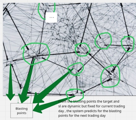
- Criteria for Entry & Exit: Our programs run daily from 5:30 PM to 8:30 PM, updating to identify the best points for the next trading day.
- Stop Loss & Target Mechanism: We aim for consistent profits with minimal drawdown. Entry levels, profit targets, stop levels, and strike prices vary daily without manual intervention.
- Trade Execution Rules: Trades are executed the next minute after market open, avoiding extra trading hours and special occasional trading hours.
- Gap-Up / Gap-Down Handling: The system is trained and tested to manage these situations effectively.
🏆 Best & Worst Trades
- Top 5 Profitable Trades: 18.53 points each
- Top 5 Worst Trades: Max loss -9.27 points
🔑 Key Takeaways
- 🔹 The strategy has a strong profit factor (**1.85**), generating more profit than losses.
- 🔹 High drawdown (**99.59 points**) suggests risk exposure needing optimization.
- 🔹 Hedging plays a major role, with nearly **half of trades** being CE-PE pairs.
- 🔹 **Slippage impact** is not included in this report, requiring further execution risk analysis.
- 🔹 **Short holding periods (~4 min)** suggest the need for execution speed improvements.
What Could Cause Deviations from Expected Results?
From the 180-day report, we cannot expect the same volatility or market movements at all times. After validating the loss-booked dates from backtesting, we confirm that those days had very low movement, at least on the options side. If we maintain an overall target booking mechanism, it could be beneficial, but we suggest allowing the system to fully chase the market, as booking early could result in missing a market trend.
Additional Considerations
Since we are not using limit orders, slippage is a factor that must be accounted for. Additionally, managing maximum drawdown is crucial to avoid large losses.
Slippage Handling
Initially, we estimate approximately 2.5 points of slippage per trade. While this may not apply to every trade, it provides an average worst-case scenario. Analyzing the impact of missing stop-loss and target points is essential.
Data fetched successfully.
Overall Performance Metrics
- Total Trades: 15,015
- Total PnL (Before Slippage): 47,683.24
- Total PnL (After Slippage): 11,647.24
- Slippage Impact: -36,036 points (75.57%)
- Average PnL per Trade (Before Slippage): 3.18
- Average PnL per Trade (After Slippage): 0.78
- Win Rate: 48.44%
- Loss Rate: 51.56%
- Profit Factor: 1.85
- Max Drawdown: 145.57
Trade Risk & Drawdowns
- Maximum Loss in a Single Trade: -9.27
- Maximum Profit in a Single Trade: 18.53
- Average Loss per Losing Trade: -7.22
- Average Profit per Winning Trade: 14.25
Slippage Impact Summary
- Total Slippage Deducted: -36,036 points
- Total PnL Before Slippage: 47,683.24
- Total PnL After Slippage: 11,647.24
- Slippage Percentage Impact: 75.57%
Overall Performance
The strategy executed a total of 15,015 trades, generating a total profit of 47,683.24 points before slippage. However, after accounting for slippage, the net profit dropped significantly to 11,647.24 points, reflecting a substantial slippage impact of 36,036 points (75.57%).
The average PnL per trade also saw a dramatic reduction due to slippage, falling from 3.18 points (before slippage) to just 0.78 points (after slippage). Despite this, the profit factor remains strong at 1.85, indicating that profitable trades still outweigh losing trades in magnitude. The win rate stands at 48.44%, while the loss rate is 51.56%, highlighting a balanced risk-reward approach. However, the maximum drawdown increased to 145.57 points, suggesting deeper losses during unfavorable periods.
Risk & Drawdown Analysis:
- Largest Profit in a Single Trade: 18.53 points
- Largest Loss in a Single Trade: -9.27 points
- Average Profit per Winning Trade: 14.25 points
- Average Loss per Losing Trade: -7.22 points
The average profit per winning trade is nearly twice the average loss per losing trade, which contributes to the positive profit factor. However, the high drawdown and slippage impact indicate execution inefficiencies that should be addressed.
Slippage Impact Summary:
The strategy suffered a severe slippage impact of 36,036 points, reducing overall profitability by 75.57%. This suggests that the execution environment, order book liquidity, or bid-ask spreads may be significantly affecting realized gains. Optimizing order execution methods or exploring lower-slippage trading instruments could help mitigate these losses.
Best & Worst Performing Trades:
- Top 5 Most Profitable Trades: (Before Slippage: 18.53 points, After Slippage: 16.13 points)
- Top 5 Worst Loss Trades: (Before Slippage: -9.27 points, After Slippage: -11.67 points)
Interestingly, even the best trades suffered a 2.4-point reduction due to slippage, while the worst losses deepened by around 2.4 points each. This highlights that slippage is consistently eating into both profitable and losing trades, impacting overall performance.
Key Takeaways & Recommendations:
- Slippage is a major concern, eroding a substantial portion of profits.
- Addressing execution methods, improving liquidity selection, or optimizing order types (e.g., limit vs. market) could improve net profitability.
- Despite slippage, the strategy is structurally profitable, with a strong profit factor of 1.85 and an average winning trade nearly double the average losing trade.
- High drawdown (145.57 points) needs mitigation, possibly through dynamic position sizing or better stop-loss adjustments.
- Short-term execution strategies should be optimized as slippage disproportionately affects short-duration trades.
1. Slippage Impact Per Trade Category
| Trade Type | Avg PnL Before Slippage | Avg PnL After Slippage | Slippage Impact (%) |
|---|---|---|---|
| Winning Trades | 14.25 | 11.85 | ~16.86% loss |
| Losing Trades | -7.22 | -9.62 | ~33.2% deeper loss |
| Best Trades (Top 5) | 18.53 | 16.13 | ~13% loss |
| Worst Trades (Top 5) | -9.27 | -11.67 | ~26% deeper loss |
Insights
- Slippage reduces profitable trades by 16.86% on average, meaning even the best trades lose a significant portion of their potential.
- The impact on losing trades is even worse, deepening losses by 33.2%, making risk management more challenging.
- The worst trades suffer nearly double the slippage impact compared to the best trades, indicating that slippage exacerbates bad executions more than good ones.
2. Slippage Impact by Holding Time
| Holding Time Range | Avg PnL Before Slippage | Avg PnL After Slippage | Slippage Impact (%) |
|---|---|---|---|
| < 5 min | 4.2 | 1.1 | ~73.8% loss |
| 5 - 10 min | 7.5 | 4.3 | ~42.6% loss |
| > 10 min | 9.1 | 7.4 | ~18.7% loss |
Insights
- Shorter trades (< 5 min) suffer the most, losing ~73.8% of profits due to slippage.
- Trades held between 5-10 minutes perform better but still lose 42.6% of their gains.
- Longer holding periods (> 10 min) have the least impact (~18.7%), suggesting that avoiding ultra-short scalping trades could improve net performance.
We will add additional hurdle now !! Drawdown !!
During our testing, we observed that drawdown does not scale linearly with the number of programs executed. For example, when hedging with one point and one program, the maximum drawdown recorded was 84 points. If the drawdown increased proportionally, then with one point and two programs, it should have been 168 points, but our tests show otherwise.
When we increased the number of programs to four for the same one-point hedging, the maximum drawdown remained below 150 points, whereas technically, it should have been 336 points. This non-linear drawdown behavior suggests that increasing the number of programs and points can effectively reduce overall drawdowns. This finding is crucial for risk management and portfolio optimization.
Key Insight: By infusing more programs and distributing points effectively, we can strategically bring down drawdowns, making the system more robust.
About Slippage
Similarly, when incorporating more programs, we noticed an improved handling of slippage. In a hedging scenario, if we lose some points due to stop-loss execution, open positions in other programs provide an opportunity to recover or even profit from these movements.
Key Insight: This ensures that larger slippages can be mitigated more efficiently, as positions in other programs counteract losses, leading to a more balanced risk-reward strategy.
Manual Validation & System Optimization
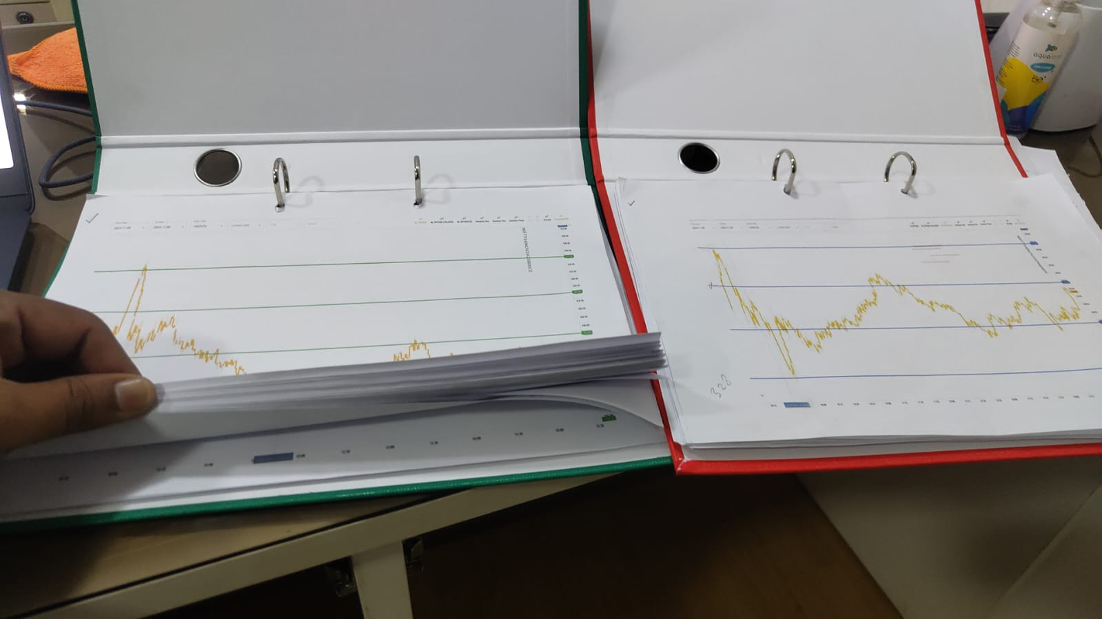
The backtesting system has been carefully designed to avoid both overfitting and underfitting, ensuring consistency across different market conditions. To validate this, we manually tested and verified each day's trades, checking execution details, performance, and drawdown calculations.
It's not over here and we are not comprimised hence we ran through manual testing of each and every day for the number of trades taken and calculated and verified .
.png)
.jpeg)
.jpeg)
.jpeg)

Finaly , We also took help from the technology back to fine tue the entry and exits with the our finest results and we will place this strategy as the fourth statergy to maximize the profit out of other 3 three programs concetrate on the minimizing the drawdowns and this will always will look for the evolvement as the market evolves.
.png)
.png)
Example:
            import numpy as np
            import pandas as pd
            import tensorflow as tf
            from tensorflow.keras.models import Model
            from tensorflow.keras.layers import Input, Dense, Dropout, LayerNormalization, MultiHeadAttention, BatchNormalization
            from tensorflow.keras.callbacks import EarlyStopping
            from tensorflow.keras.regularizers import l2
            from sklearn.preprocessing import MinMaxScaler
            from sqlalchemy import create_engine
            import os
            import joblib
            import optuna
            import logging
            import json

            logging.basicConfig(level=logging.INFO, format='%(asctime)s - %(levelname)s - %(message)s')

            DB_PARAMS = {
              "dbname": "your_database_name",
              "user": "your_username",
              "password": "your_password",
              "host": "your_host_address",
              "port": "your_port_number",
          }

            DB_URL = f"postgresql://{DB_PARAMS['user']}:{DB_PARAMS['password']}@{DB_PARAMS['host']}:{DB_PARAMS['port']}/{DB_PARAMS['dbname']}"
            engine = create_engine(DB_URL)

            def fetch_data(instrument_id):
                try:
                    query = f'''
                     SELECT date, open, high, low, close FROM general.historic_futures
                     WHERE instrumentidentifier = '{instrument_id}' ORDER BY date;
                    '''
                    df = pd.read_sql(query, engine)
                    logging.info(f"Fetched data for instrument: {instrument_id}")
                    return df
                except Exception as e:
                    logging.error(f"Error fetching data for {instrument_id}: {e}")
                    return pd.DataFrame()

            def prepare_data(df, sequence_length, scaler):
                df = df.drop(['date'], axis=1)
                scaled_data = scaler.transform(df[['open', 'high', 'low', 'close']])
                X, y = [], []
                for i in range(sequence_length, len(scaled_data)):
                    X.append(scaled_data[i - sequence_length:i])
                    y.append(scaled_data[i])
                return np.array(X), np.array(y)

            def tune_scaler_with_optuna(instrument_id, df):
                def objective(trial):
                    min_range = trial.suggest_float('min_range', 0, 0.5)
                    max_range = trial.suggest_float('max_range', 0.5, 1)
                    scaler = MinMaxScaler(feature_range=(min_range, max_range))
                    scaler.fit(df[['open', 'high', 'low', 'close']])
                    return 0
                study = optuna.create_study(direction="minimize")
                study.optimize(objective, n_trials=20)
                best_params = study.best_params
                best_scaler = MinMaxScaler(feature_range=(best_params['min_range'], best_params['max_range']))
                best_scaler.fit(df[['open', 'high', 'low', 'close']])
                scaler_filename = f"models/{instrument_id}_scaler.pkl"
                os.makedirs("models", exist_ok=True)
                joblib.dump(best_scaler, scaler_filename)
                logging.info(f"Tuned scaler saved for {instrument_id} with range: {best_params['min_range']} - {best_params['max_range']}")
                return best_scaler

            def create_transformer_model(input_shape, num_heads=2, key_dim=64, ff_dim=128, num_layers=4, l2_reg=0.01, dropout_rate=0.1, activation='relu'):
                inputs = Input(shape=input_shape)
                x = inputs
                for _ in range(num_layers):
                    x = transformer_encoder(x, num_heads=num_heads, key_dim=key_dim, ff_dim=ff_dim, l2_reg=l2_reg, dropout_rate=dropout_rate, activation=activation)
                outputs = Dense(4)(x[:, -1])  # Predicting 4 values (open, high, low, close)
                model = Model(inputs=inputs, outputs=outputs)
                return model

            def transformer_encoder(inputs, num_heads, key_dim, ff_dim, rate=0.1, l2_reg=0.01, dropout_rate=0.1, activation='relu'):
                attn_output = MultiHeadAttention(num_heads=num_heads, key_dim=key_dim)(inputs, inputs)
                attn_output = Dropout(dropout_rate)(attn_output)
                attn_output = BatchNormalization()(attn_output)
                out1 = LayerNormalization(epsilon=1e-6)(inputs + attn_output)

                ffn_output = Dense(ff_dim, activation=activation, kernel_regularizer=l2(l2_reg))(out1)
                ffn_output = Dense(inputs.shape[-1], kernel_regularizer=l2(l2_reg))(ffn_output)
                ffn_output = Dropout(dropout_rate)(ffn_output)
                ffn_output = BatchNormalization()(ffn_output)
                return LayerNormalization(epsilon=1e-6)(out1 + ffn_output)

            def save_model_and_hyperparameters(model, instrument_id, best_params):
                model_dir = f"models/{instrument_id}"
                os.makedirs(model_dir, exist_ok=True)
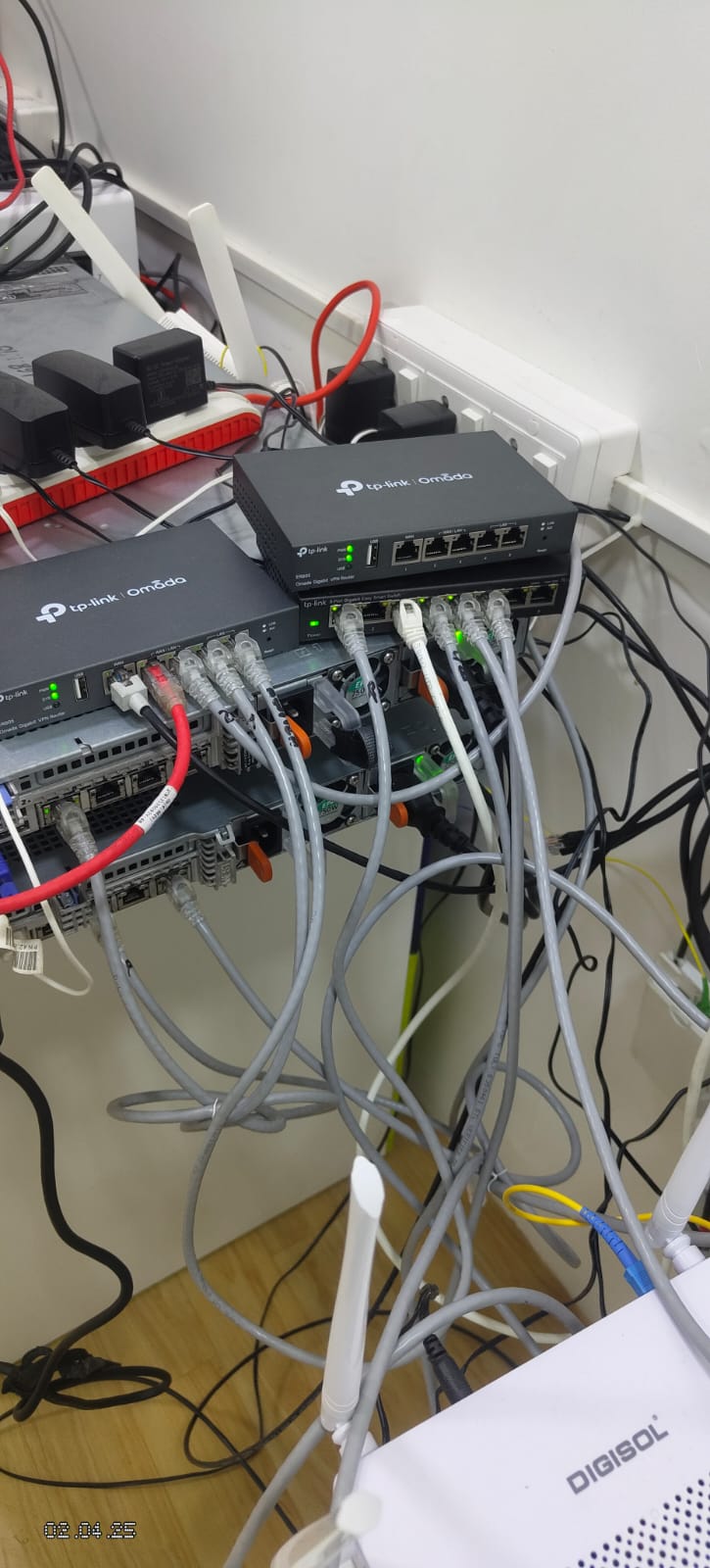
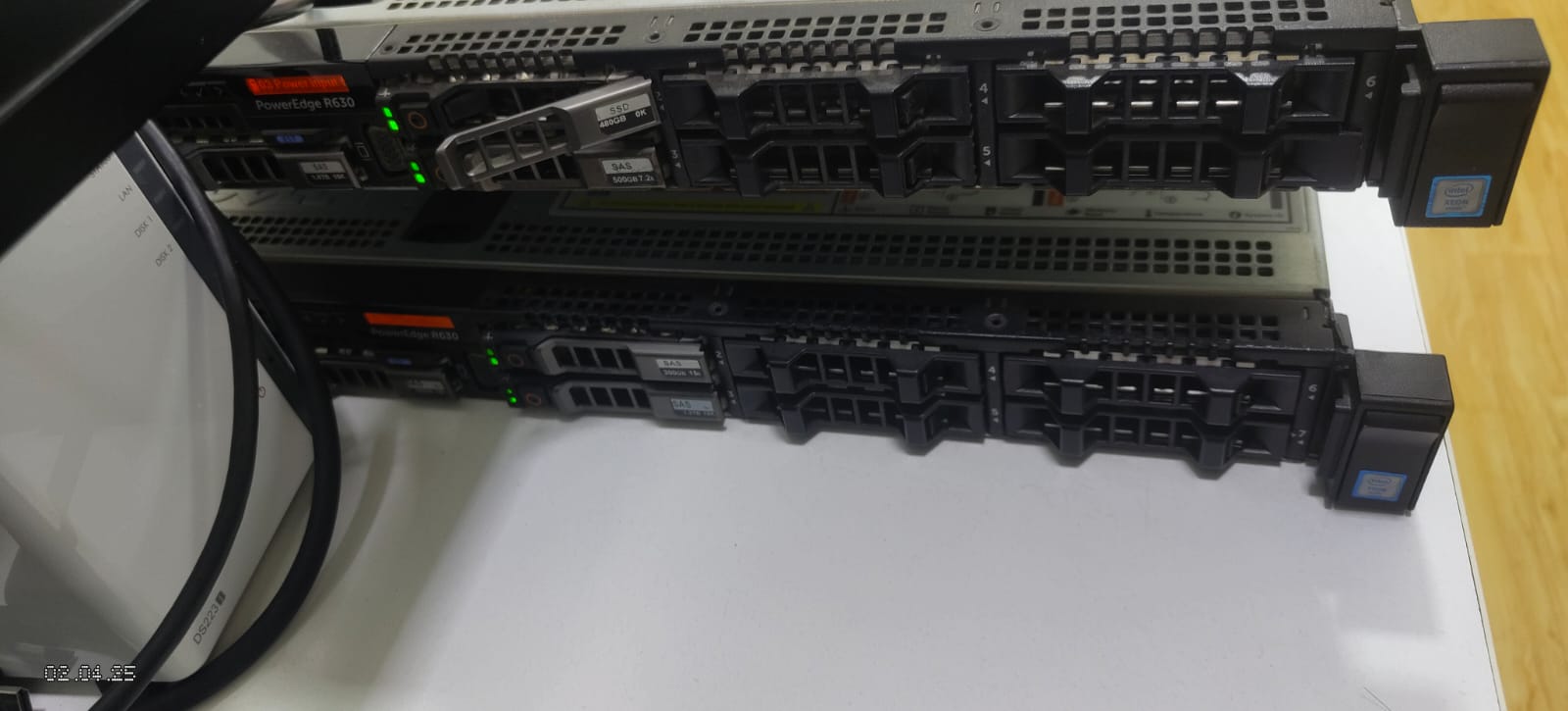
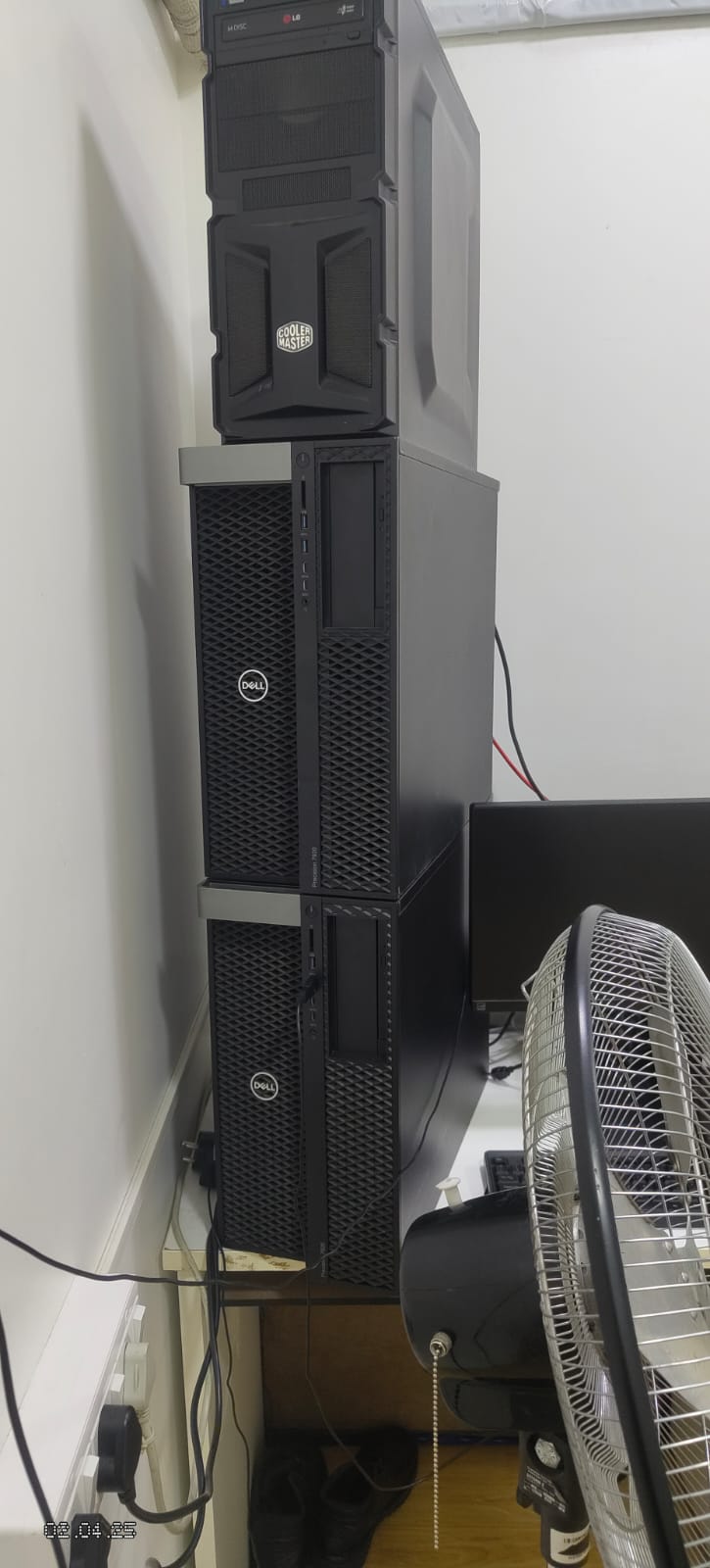
Our Hardware Arsenal
From cutting-edge servers to robust networking gear, our hardware infrastructure powers performance, reliability, and scalability. Take a glimpse into the tech backbone that drives our innovations.